6. Additive, Subtractive, & Modulation Synthesis

SC has a built in spectrum analyzer that is a useful tool for monitoring your sound design work, particularly during the development stage. Run the following line:

FreqScope.new;

and then proceed through the rest of this lab.

Additive Synthesis

Additive Synthesis is the technique of combining multiple sounds to create more complexity. We went over a simple example as part of this lab on Tuesday:

{ SinOsc.ar( 440, 0.0, 0.5 ) + PinkNoise.ar( 0.1 ) + Crackle.ar( 1.5, 0.4 ) + LFTri.ar( 200, 0.0, 0.2 )}.play;

Here we "sum," or add, signals together to create a complex sound from two oscillators (SinOsc and LFTri) and two noise generators (PinkNoise and Crackle).

Another example of additive synthesis can be seen below:

{SinOsc.ar(800,0,0.1) + SinOsc.ar(880,0,0.1)}.scope;

Here we sum two Sine tones to simulate the busy sound heard on old telephones. This is a good example of another additive synthesis technique: summing multiples of the same sound to create more complex sounds.

SC has a nice shortcut for the above, so one can rewrite it as follows:

{SinOsc.ar([800,880],0,0.1)}.scope;

This takes advantage of a cool feature of Supercollider: Multichannel Expansion. When the Server sees an argument with an Array as input it duplicates the Synth for every item in that Array, explaining why the two previous examples are effectively the same (though one requires less typing!).

Mix

Mix can be used to combine an Array of sounds and mix them down to Mono. For example:

SynthDef( \addSynth,    { | amp = 0.0, freq = 440, out = 0, phase = 0.0, trig = 0 |
    var env, sig, finalSig;
    env = EnvGen.kr( Env.asr( 0.001, 0.9, 0.001 ), trig, doneAction: 0 );
    sig = Mix( [ SinOsc.ar( freq, phase, 0.5 ), PinkNoise.ar( 0.1 ), Crackle.ar( 1.5, 0.4 ), LFTri.ar( freq/2, phase, 0.2 )]);
    finalSig = sig * env * 0.6;
    Out.ar( out, Pan2.ar(finalSig) );
}).add;

x = Synth( \addSynth, [\amp, 0.5, \trig, 1]); // instantiate and play the synth

x.set(\trig, 0); // stop playing the synth when you have had enough

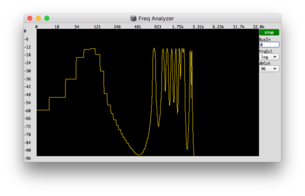
Another application of Mix, and also an example of using many SinOscs to create a complex sound, is provided by Mix.fill: one can generate and fill an array of signals. For example, the following Synth creates 16 instances of SinOsc and then mixes them down to one Mono signal:

SynthDef( \addSynth, { | amp = 0.0, freq = 440, out = 0, phase = 0.0, trig = 0 |
    var env, sig, finalSig;
    env = EnvGen.kr( Env.asr( 0.001, 0.9, 0.001 ), trig, doneAction: 0 );
    sig = Mix.fill(16, {SinOsc.ar(rrand(100, 3000), 0.0, amp)});
    finalSig = sig * env * 0.6;
    Out.ar( out, Pan2.ar(finalSig) );
}).add;

x = Synth( \addSynth, [\amp, 0.5, \trig, 1]); // instantiate and play the synth

x.set(\trig, 0); // stop playing the synth when you have had enough

Which looks like this in the FreqScope:

Subtractive Synthesis

Subtractive Synthesis is analogous to sculpting something out of marble with a hammer and chisel: we start with a complex sound and carve out parts of it to produce a different sound. In general Subtractive Synthesis relies on various Filters to accomplish this transformation. For example, let's start with a PinkNoise generator (remember to run FreqScope again if you turned it off):

x = {| amp = 0.1 | PinkNoise.ar(amp) }.play;

Free the synth (x.free;) and then run this:

x = {| amp = 0.1, freq = 1000 | LPF.ar(PinkNoise.ar(amp), freq, amp) }.play;

Here we run the PinkNoise generator from the previous example through a Low Pass Filter (LPF in SC), which will only allow parts of the sound below a set frequency through. Free the Synth and run again with a few different frequencies, noting the difference in sound.

A High Pass Filter (HPF in SC) is the opposite of a LPF. Compare the previous example with the following:

x = {| amp = 0.1, freq = 1000 | HPF.ar(PinkNoise.ar(amp), freq, amp) }.play;

Here we only allow parts of the sound with frequencies above 1000Hz through. Note that because we are filtering out the lower, stronger sounding frequencies our resulting sound ends up seeming low in volume. It is normal to scale all other sounds down accordingly to achieve balance if the low volume of the filtered audio is problematic.

A Band Pass Filter (BPF in SC) can filter an input by defining the quantity of frequencies, below and above, allowed to pass around a center frequency. To hear the effect, first run our dry PinkNoise Synth:

x = {| amp = 0.1 | PinkNoise.ar(amp) }.play;

Free the synth (x.free;) and then run this:

x = {| amp = 0.1, freq = 1000, rq = 0.1 | BPF.ar(PinkNoise.ar(amp), freq, rq, amp) }.play;

The lower the rq the less frequencies are allowed to pass around the center frequency. To experience this difference try running the above example a few times with different rq values (note: rq can be a number between 0.0 and 1.0 but setting it to 0.0 is equivalent to turning the Synth off and setting it to 1.0 is equivalent to not using the filter at all).

Modulation Synthesis

Modulation Synthesis refers to the technique of using a time-varying signal, called the modulator, to influence or change the behavior of another time-varying signal, called the carrier. Interestingly enough, we can use this technique to modulate the frequency, phase, or amplitude of a time-varying signal to produce different effects.

A classic example of this technique, called Ring Modulation:

SynthDef( \ringMod, { | amp = 0.0, out = 0, trig = 0|
    var carrier, carrfreq, env, modulator, modfreq, sig;

    env = EnvGen.kr( Env.asr( 0.001, 0.9, 0.001 ), trig, doneAction: 0 );
    carrfreq = MouseX.kr(440,5000,'exponential');
    modfreq = MouseY.kr(1,5000,'exponential');
    carrier= SinOsc.ar(carrfreq,0,0.5);
    modulator= SinOsc.ar(modfreq,0,0.5);
    sig = carrier * modulator * env;
    Out.ar(out, Pan2.ar(sig))
}).add;

x = Synth( \ringMod, [ \amp, 0.5, \trig, 1 ]);

An example of Amplitude Modulation:

SynthDef( \ampMod, { | amp = 0.0, out = 0, trig = 0|
    var carrier, carrfreq, env, modulator, modfreq, sig;

    env = EnvGen.kr( Env.asr( 0.001, 0.9, 0.001 ), trig, doneAction: 0 );
    carrfreq = MouseX.kr(440,5000,'exponential');
    modfreq = MouseY.kr(1,5000,'exponential');
    carrier= SinOsc.ar(carrfreq,0,0.5);
    modulator= SinOsc.ar(modfreq,0,0.25, 0.25);
    sig = carrier * modulator * env;
    Out.ar(out, Pan2.ar(sig))
}).add;

x = Synth( \ampMod, [ \amp, 0.5, \trig, 1 ]);

Since we are modulating amplitude, in the above, we can only use positive numbers. This is done by adding 0.25 to the input, so the modulator never drops below 0.0.

And finally (for now), Frequency Modulation:

SynthDef( \freqMod, { | amp = 0.0, out = 0, trig = 0 |
    var env, modfreq, modindex, sig;

    env = EnvGen.kr( Env.asr( 0.001, 0.9, 0.001 ), trig, doneAction: 0 );
    modfreq = MouseX.kr(1,440, 'exponential');
    modindex = MouseY.kr(0.0,10.0);
    sig = SinOsc.ar(SinOsc.ar(modfreq,0,modfreq*modindex, 440),0,amp) * env;
    Out.ar( out, Pan2.ar(sig));
}).add;

x = Synth( \freqMod, [ \amp, 0.5, \trig, 1 ]);